spatial_packages <- c(
  "arcpullr", "dplyr", "ggplot2", "ggspatial",
  "leaflet", "rnaturalearth", "sf", "terra"
)
optional_packages <- c("ckanr")

spatial_ready <- all(vapply(spatial_packages, requireNamespace, FUN.VALUE = logical(1), quietly = TRUE))
ckan_ready <- all(vapply(optional_packages, requireNamespace, FUN.VALUE = logical(1), quietly = TRUE))

if (!spatial_ready) {
  missing <- spatial_packages[!vapply(spatial_packages, requireNamespace, FUN.VALUE = logical(1), quietly = TRUE)]
  message("Skipping spatial execution; missing packages: ", paste(missing, collapse = ", "))
}
if (!ckan_ready) {
  message("Skipping CKAN examples; package 'ckanr' is not installed.")
}Accessing Spatial Data from the Open Government Portal
Background
This tutorial provides an overview for how to extract spatial data from the Open Government Portal, commonly referred to as Open Data. OGP is the Government of Canada’s official platform for publishing federal datasets, and DFO Science staff publish eligible data products there to meet open data policy requirements, ensure visibility of our work, and support reuse by partners and the public.
The code below shows how to leverage the resources available on OGP, making it easier to meet FAIR (Findable, Accessible, Interoperable, Reusable) principles and support reproducible science.
This tutorial reviews:
Querying ArcGIS REST services
Extracting data from file geodatabases
Using
ckanrto build more robust code
The examples cover the basics of mapping in R, including plotting both vector and raster data with ggplot(), and creating leaflet maps. Many online tutorials provide further detail for specifics of mapping in R if you need more background. For example, this tutorial from the University of Toronto provides a very good overview.
Note that much of this content has been expanded from a similar tutorial created in the DFO Maritimes Region, but with DFO Pacific examples. Other clarifying comments have also been added.
Loading packages
This tutorial uses several spatial packages that require system libraries. If those dependencies are not installed locally, code chunks are skipped so site rendering can still complete. Static map outputs are cached under images/openDataSpatial/rendered/ so published pages keep map images even when spatial dependencies are unavailable.
Note: Spatial code examples are skipped in this render because required system dependencies are not installed locally. Note: CKAN API examples are skipped in this render because
ckanris not installed.
Accessing Open Data via ARCGIS REST
The arcpullr package is a great way to access ArcGIS REST services, which are often used for storing spatial data on Open Data. You can use the get_spatial_layer() function to retrieve a spatial layer from an ArcGIS server.
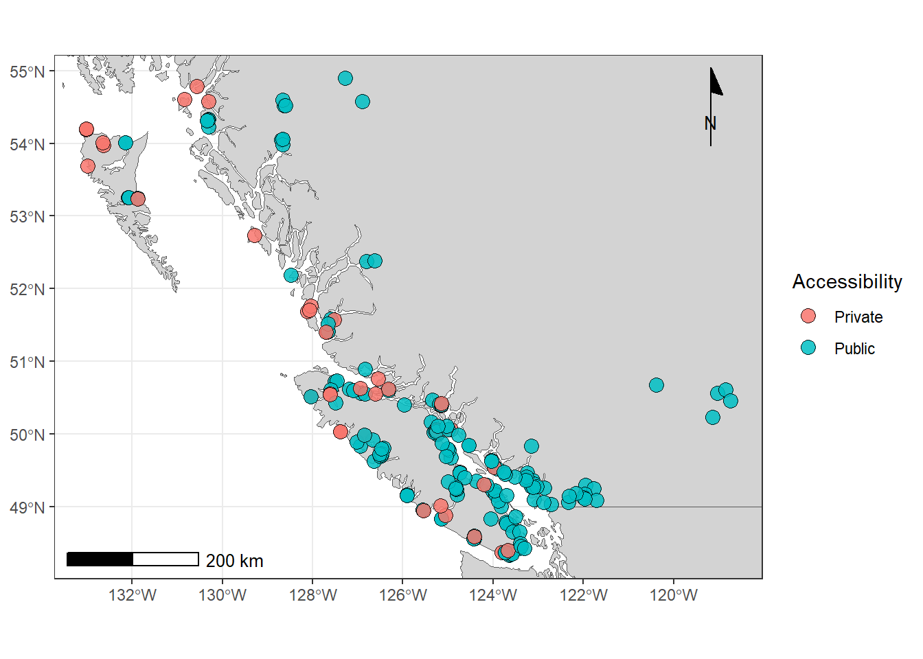
Example: Pacific Recreational Fishery Salmon Head Depots
There can many URLs associated with each dataset. The “ArcGIS Rest URL” we need to feed into the get_spatial_layer() function should be the one that includes “arcgis/rest/services”.
For example, with the Pacific Recreational Fishery Salmon Head dataset, the URL we are interested in is https://egisp.dfo-mpo.gc.ca/arcgis/rest/services/open_data_donnees_ouvertes/pacific_recreational_fishery_salmon_head_depots/MapServer/.
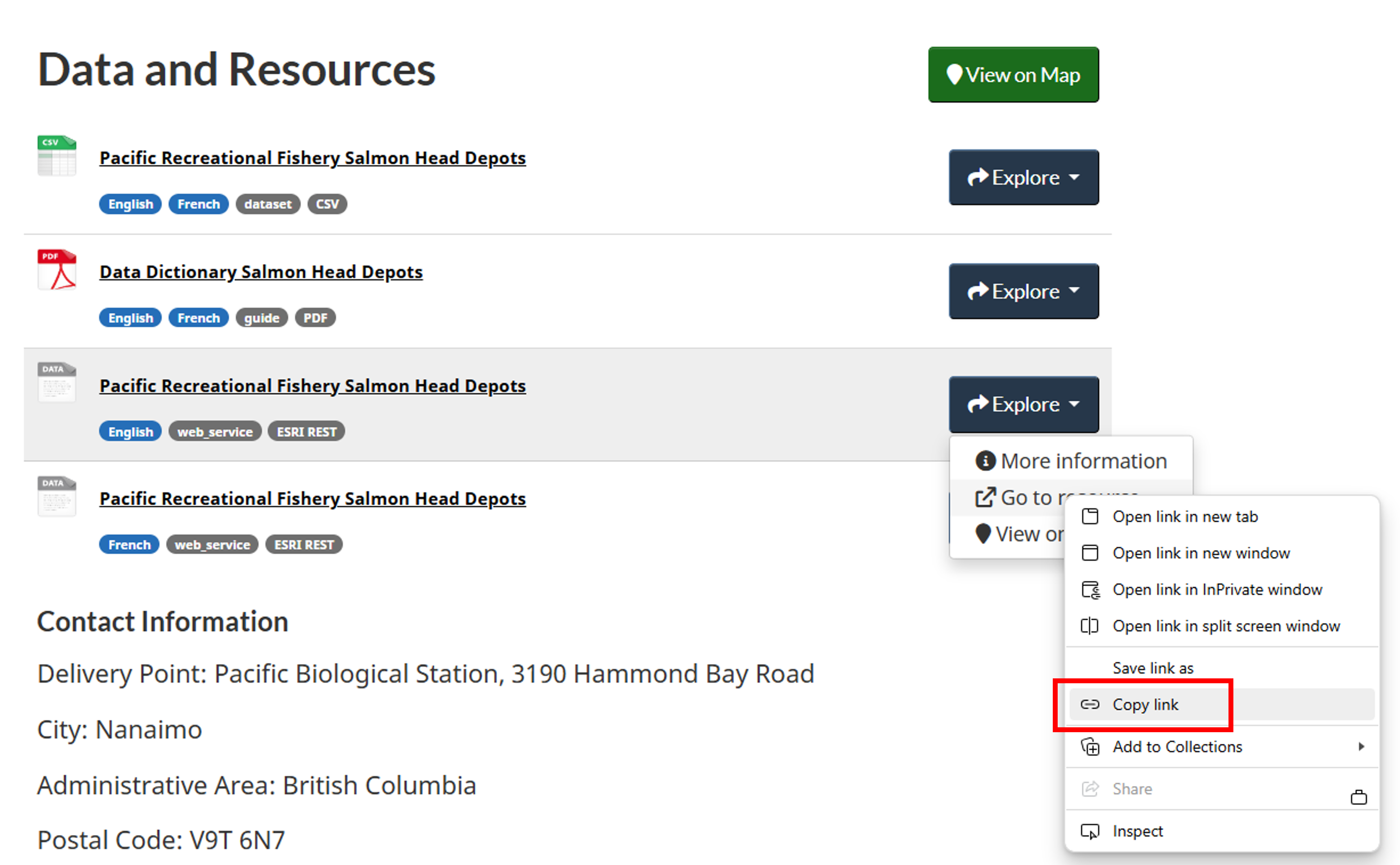
If you have trouble tracking this down, go to the appropriate dataset page on Open Data.
Then, under the Data and Resources section, find the item labelled ESRI REST (there is both an English and French example). Left click on the Explore dropdown item, then right click on Go to resource, and then left click on Copy link. This then copies the link to the URL you need.
It is important to ensure the appropriate layer is specified. In this example, the “0” at the end of the address denotes the English version, while a 1 represents French (see layers within the MapServer page). They also do not always correspond to language. For example, in the Pacific Commercial Salmon In Season Catch Estimates dataset, layers 0 to 3 represent gill nets, troll, seine and Pacific Fishery Management Areas, respectively.
salmonDepots = arcpullr::get_spatial_layer("https://egisp.dfo-mpo.gc.ca/arcgis/rest/services/open_data_donnees_ouvertes/pacific_recreational_fishery_salmon_head_depots/MapServer/0")Creating a map
There are some great packages to get basemaps in R. The rnaturalearth package is a good option for getting country borders and other geographical features. You can use the ne_countries() function to get country borders.
In British Columbia, rnaturalearth may not have the level of detail required (e.g., some islands are missing). The bcmaps package has a lot of detailed basemaps and spatial data for the BC coast, and the bc_bound_hres() function is particularly useful for mapping coastline.
Since the data used in the tutorial are for the entire BC coast, rnaturalearth is used in the examples below.
# Get coastline for North America
coast = ne_countries(scale = 10, returnclass = c("sf"), continent = "North America")
Because the coastline basemap data span all of North America, it may be useful to crop the plot to the bounding box of the data (BC coast). The st_bbox() function from the sf package allows you to get the bounding box of a spatial object. You can use the xlim and ylim arguments in the coord_sf() function to set the limits of the x and y axes.
Accessing file geodatabases
File geodatabases are a proprietary file format developed by ESRI for spatial and non-spatial data. Many spatial datasets are uploaded to Open Data as file geodatabases, and it is possible to download and extract them with R!
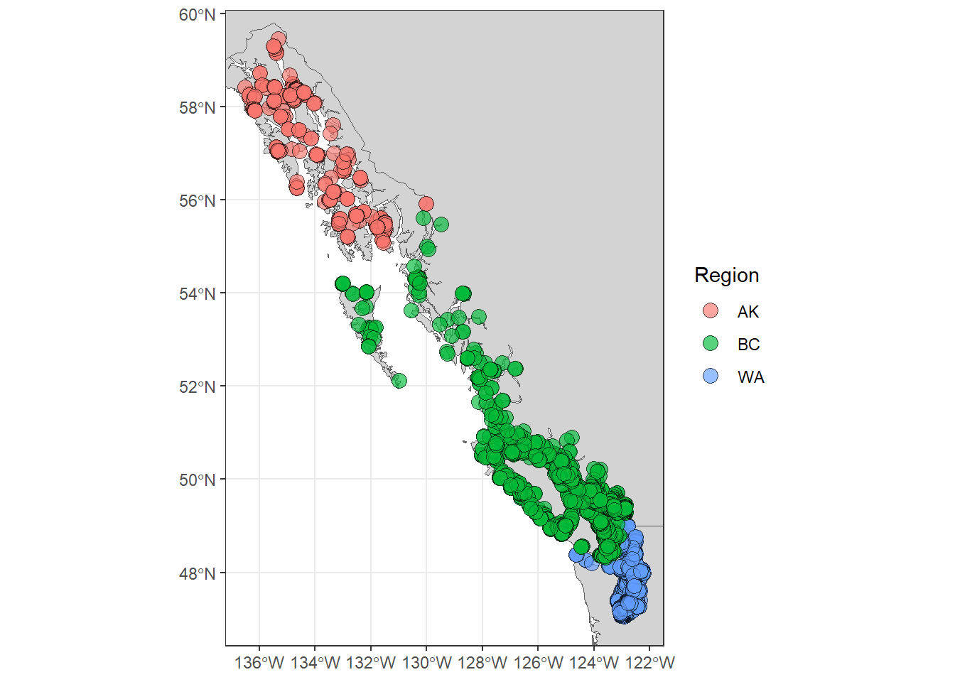
The example below shows how to access the file geodatabase from the floating infrastructure dataset on Open Data
Creating temporary directories
For exploring data, it is often helpful to create temporary directories to store and extract data. This can be easier than downloading the data directly and setting your directories.
# Create a temporary directory to store the downloaded zip file
temp_dir = tempdir()

# Define the path for the downloaded zip file inside the temp directory
zip_file = file.path(temp_dir, "zipPath.gdb.zip")

# Define the directory where the zip contents will be extracted
# This is a relative path, so files will be extracted into the current working directory
unzip_dir = file.path("extracted_fgdb")

# Download the dataset zip file. To get the correct link, follow the same steps as in the Pacific Recreational Fishery Salmon Head Depots example above, but with the "FDGB/GDB" item in Data and resources
download.file(
  "https://api-proxy.edh-cde.dfo-mpo.gc.ca/catalogue/records/049770ef-6cb3-44ee-afc8-5d77d6200a12/attachments/floating_infrastructure-docks.gdb.zip",
  destfile = zip_file,
  mode = "wb"
)

# Create the extraction directory if it doesn't already exist
dir.create(unzip_dir, showWarnings = FALSE)

# Unzip the downloaded file into the extraction directory
unzip(zip_file, exdir = unzip_dir)

# List the files extracted to verify contents
list.files(unzip_dir)

# Load the layers available in the extracted .gdb file
# Copy the name from the list.files() command. This should match the name of the gdb from the URL above
layers = st_layers(file.path(unzip_dir, "floating_infrastructure-docks.gdb"))

# Turn layers from a list into a dataframe
# layers has 1 entry called docks, so now a df called 'docks' will be created
for(l in layers$name){
  message("Reading layer: ", l)
  assign(l, st_read(file.path(unzip_dir, "floating_infrastructure-docks.gdb"), layer = l, quiet = TRUE))
}
Map the data
Plotting raster data
An example is shown here for accessing and plotting raster data stored in a geodatabase. You can follow the example in the Maritimes tutorial for accessing raster data from tiff files, if you are interested.
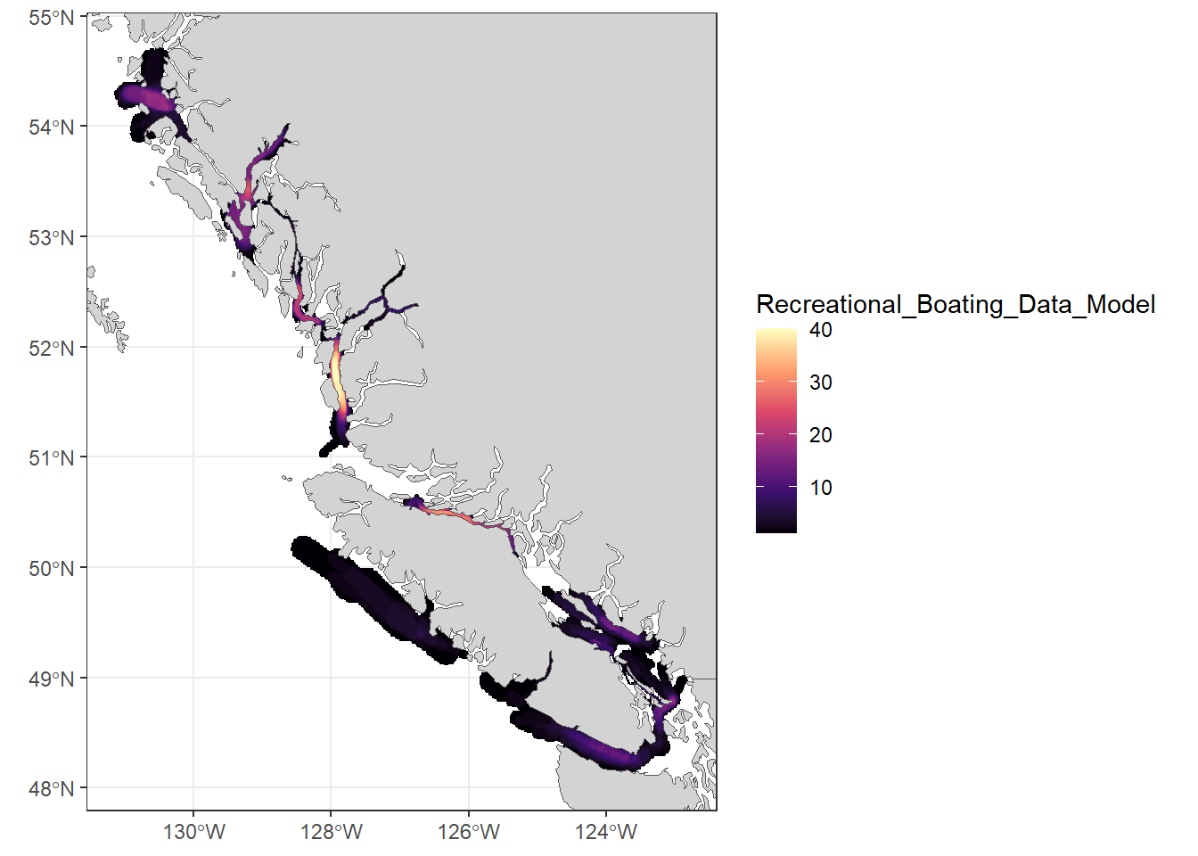
The example I’m using is from the recreational vessel traffic model on the BC coast.
# Follow steps above to create a temporary folder to download & extract geodatabase info
temp_dir = tempdir()
zip_file = file.path(temp_dir, "bc_boating_model.zip")
unzip_dir = file.path(temp_dir, "bc_boating_data")

# Download the dataset zip file. To get the correct link, follow the same steps as in the Pacific Recreational Fishery Salmon Head Depots example above, but with the "FDGB/GDB" item in Data and resources
download.file(
  url = "https://api-proxy.edh-cde.dfo-mpo.gc.ca/catalogue/records/fed5f00f-7b17-4ac2-95d6-f1a73858dac0/attachments/Recreational_Boating_Data_Model.gdb.zip",
  destfile = zip_file,
  mode = "wb"
)

# Unzip the contents
dir.create(unzip_dir, showWarnings = FALSE)
unzip(zip_file, exdir = unzip_dir)

# List the file names you just downloaded
boat_file = list.files(unzip_dir, full.names = TRUE)
Mapping the survey effort data with ggplot
Unfortunately, raster data in this format cannot be directly mapped with ggplot. But, you can convert it to a data frame and keep the coordinate positions.
If you read through the metadata, you’ll see that that many types of data are available in this geodatabase (e.g., point data, raster, vector grid). The data being plotted in this example below is the surveyeffort raster dataset, which is specified using the sub argument in the rast() function.
Making Leaflet Maps
Leaflet maps are interactive maps that can be a great way to explore data. Leaflet maps can also be great for point data, since you can create popup labels where you can click and view your attribute data.
# Convert raster to leaflet-compatible format
pal = colorNumeric(palette = "magma", domain = values(rast_proj), na.color = "transparent")

# Create leaflet map
leaflet() %>%
  addProviderTiles(providers$Esri.OceanBasemap) %>%
  addRasterImage(rast_proj, colors = pal, opacity = 0.7, project = T) %>%
  addLegend(pal = pal, values = values(rast_proj),
            title = "Survey Effort",
            position = "bottomright")
Using ckanr to build more robust code
Sometimes, IT needs to upgrade server hardware or software, which can result in changes to the ArcGIS REST service URLs (i.e., the portion like this: https://egisp.dfo-mpo.gc.ca/arcgis/rest/services). However, the Universally Unique Identifier (UUID) associated with each dataset remains unchanged.
In the Open Data portal, the UUID is the final part of the URL after “dataset”. For example, in the Pacific Recreational Salmon Head Depots dataset (https://open.canada.ca/data/dataset/3cc03bbf-d59f-4812-996e-ddc52e0ba99e), the UUID is 3cc03bbf-d59f-4812-996e-ddc52e0ba99e.
To make our script more robust, we can use the CKAN API. CKAN is a data management system that supports publishing, sharing, and discovering datasets. The ckanr package in R allows us to interact with CKAN-based portals, such as Open Data. You can use the ckanr_setup() function to establish a connection.
Instead of hardcoding the ArcGIS REST URL in our script (which may change) we can use the CKAN API to reference the stable UUID. This allows us to dynamically retrieve the current ArcGIS REST URL associated with that UUID, ensuring our code remains functional even if updates occur.
Downloading data
We’ll use the Pacific Recreational Fishery Salmon Head Depots data as an example. We can use the ckanr package to extract the ArcGIS REST URL by referencing the UUID. This may seem like an extra step while you’re writing your code, but it will save you time in the long run if the URLs change (it can happen!!)
ckanr::ckanr_setup("https://open.canada.ca/data")
uuid = "3cc03bbf-d59f-4812-996e-ddc52e0ba99e"
pkg = ckanr::package_show(uuid)
resources = pkg$resources
df_resources = as.data.frame(do.call(rbind, resources))

# Now you can grab the correct ESRI Rest URL ("url"). Make sure to search for that format, and also specify you want the English ("En") version and not French
salmon_url = unlist(df_resources[df_resources$format == "ESRI REST" & sapply(df_resources$language, function(x) "en" %in% x), "url"])
Searching for data
You can also use the ckanr package to search for data using the package_search() function. You can use the q argument to search for key words, and the fq argument to specify file types.
ckanr::ckanr_setup("https://open.canada.ca/data")
search_results = ckanr::package_search(q = "Pacific salmon")
search_results # Note that UUID also shows up here after the <CKAN Package> text

# You  can also search specifically for spatial data (e.g., shapefiles, geodatabases, etc.) by specifying the fq argument
search_results = ckanr::package_search(
  q = "Pacific salmon",
  fq = 'res_format:(SHP OR GDB OR GeoJSON OR KML OR CSV)' # CSVs sometimes contain spatial data, sometimes not
)